How to Read Csv Files in Jupyter Notebook Without Panda

Live Graph Simulation using Python, Matplotlib and Pandas

Make live graphs with dynamic line, scatter and bar plots. Also learn to plot graphs in 3D and 2nd quickly using pandas and csv.

Bamboozling Graphs

Pandas and Matplotlib are very useful libraries when information technology comes to graph plotting and circulation. Often it becomes quite time consuming when you have collected chunks of data but have to separately search for plotting tools to visualize your data. Pandas, coupled with matplotlib offers seamless visualization of data directly from csv files.
In this post we will learn how to plot diverse plots direct from csv files and then later how to present the data in a live moving and dynamic graph. Further equally a bonus, plotting the data in 3D shall also be described.

Lets begin coding folks

Plot direct from CSV files:

Let united states brainstorm with the basics which is past plotting unlike types of plots direct from csv files.

          import pandas as pd
import matplotlib.pyplot every bit plt        

We import the two essential packages required for the plots. For the purpose of demonstration we shall be using the csv file available hither : Link . We shall use sales records every bit it it more data centric. (CSV file)

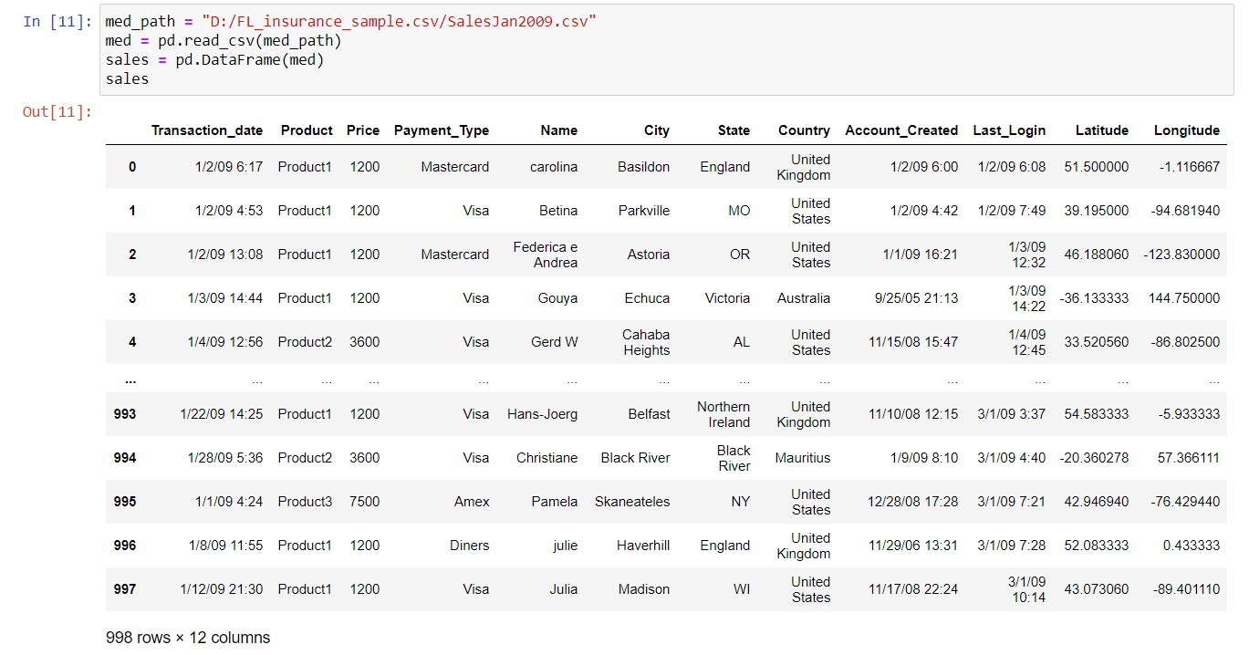
          med_path = "D:/FL_insurance_sample.csv/SalesJan2009.csv"
med = pd.read_csv(med_path)
sales = pd.DataFrame(med)
sales        

We ascertain the path of the csv file and and so using pandas read the file. Next we convert it to a pandas dataframe which makes easier to play with data. Then we visualize to see what data are we dealing with which looks something like this:

Jupyter notebook offers more than flexibility in coding

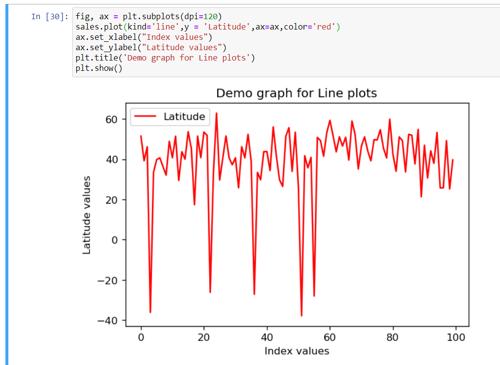
Adjacent step is to plot the data. We start with a line chart with the following snippet:

          ax =plt.gca()
sales.plot(kind='line',y = 'Latitude',ax=ax,color='red')
ax.set_xlabel("Index values")
ax.set_ylabel("Latitude values")
plt.title('Demo graph for Line plots')
plt.show()        

plt.subplots(dpi=120) gives the figure and axes for the plots while dpi helps usa decide the quality of the graph image. We describe the type of graph in kind variable so subsequently set 10 and y labels along with the plot title. Nosotros have the following output:

Linear plot for merely one entity

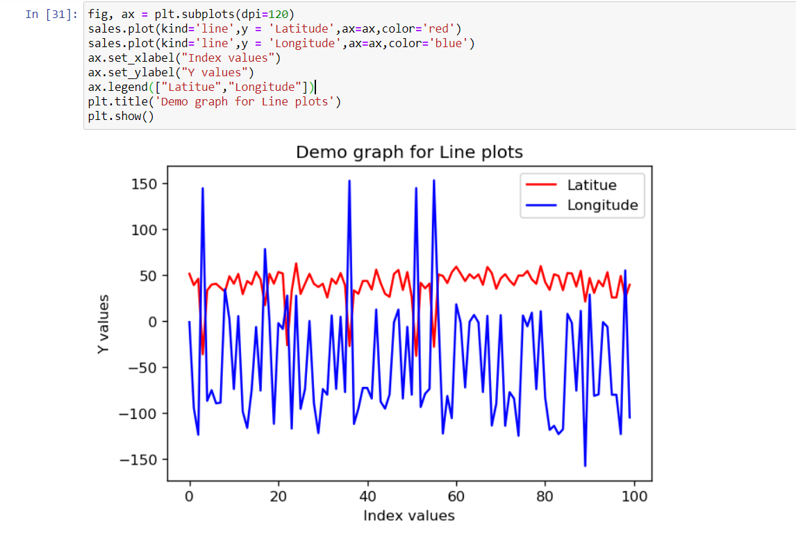
We tin can plot multiple entities by just adding more plot values along with legends for the same every bit shown below:

Keep separating the colour for each plot for ameliorate visualization

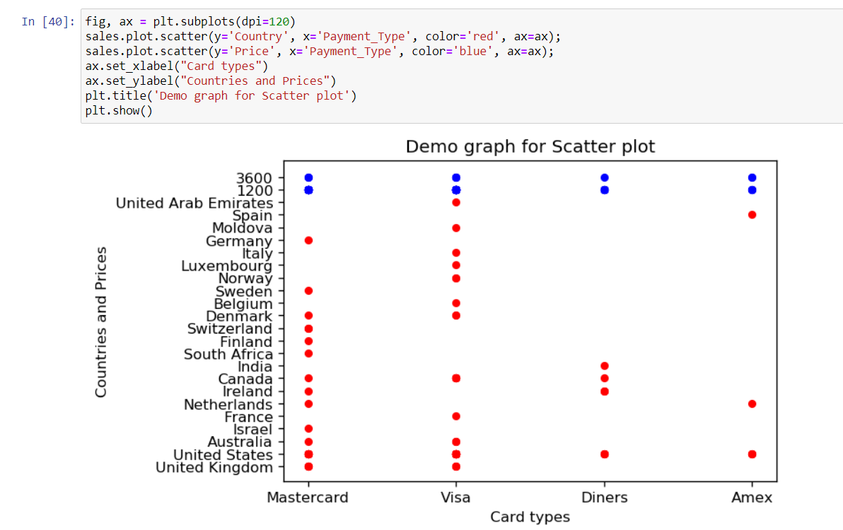
Similarly nosotros also visualize scatter plot-single plot using the post-obit snippet:

          fig, ax = plt.subplots(dpi=120)
sales.plot.scatter(y='Country', 10='Payment_Type', color='cerise', ax=ax);
ax.set_xlabel("Card types")
ax.set_ylabel("Countries")
plt.championship('Demo graph for Scatter plot')
plt.show()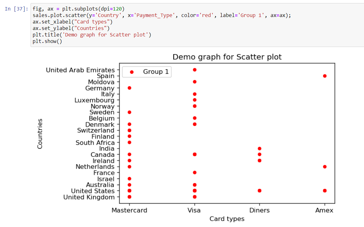        

Unmarried variable scatter plot

We and then extend for multi scatter plot in the same figure as follows:

Multi variable besprinkle plot

The data file chosen isn't very suitable for some types of plots so we use random values for better visualization for those types of plots.

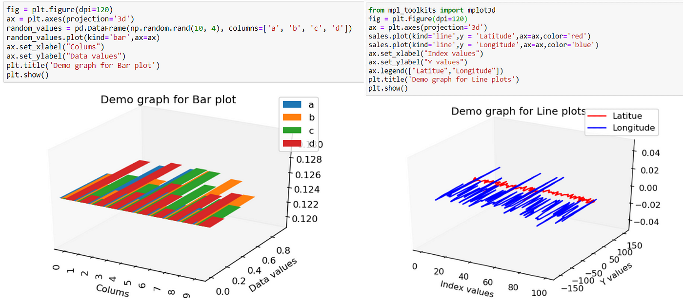
Bar Plots:

          fig, ax = plt.subplots(dpi=120)
random_values = pd.DataFrame(np.random.rand(10, 4), columns=['a', 'b', 'c', 'd'])
random_values.plot(kind='bar',ax=ax)
ax.set_xlabel("Colums")
ax.set_ylabel("Data values")
plt.title('Demo graph for Bar plot')
plt.evidence()        

Multi bar Plots in one figure

Area Plot:

          fig, ax = plt.subplots(dpi=120)
expanse = pd.DataFrame(np.random.rand(10, 4), columns=['a', 'b', 'c', 'd'])
surface area.plot(kind='area',ax=ax)
plt.title('Demo graph for Expanse plot')
plt.evidence()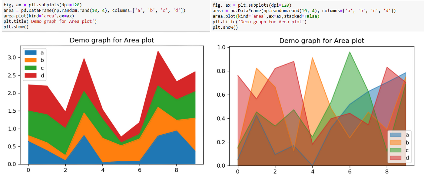        

Ii dissimilar Areas plots with stacked True and Simulated for ameliorate clarification of data

These were some of the most ordinarily used plots for data visualization. Now nosotros move on to plotting these plots every bit live and dynamic data

No long codes and so don't worry. The all-time is nevertheless to come

Alive — Dynamic Graphs:

We will be using FuncAnimation function in matplotlib for this purpose which makes blitheness by repeatedly calling a function *func*.
We ascertain the necessary imports and initializations necessary for the code execution here:

          import random
from itertools import count
import fourth dimension
import matplotlib.pyplot as plt
from matplotlib.blitheness import FuncAnimation
from mpl_toolkits import mplot3d          plt.style.use('fivethirtyeight')          x_values = []
y_values = []
z_values = []
q_values = []          counter = 0          index = count()        

We shall be plotting three dynamic line plots in the same figure and will randomly pool these values from a specified range

Firstly nosotros define the *func* role to be utilized here:

The comments in the code make it relatively easier to understand the concept that animate function keeps calling the part defined by us and plt.cla keeps refreshing the plot which makes information technology dynamic. Finally nosotros telephone call the above function to see the dynamic graphs-
fig, ax = plt.subplots()

          ani = FuncAnimation(plt.gcf(), animate, 1000)
plt.tight_layout()
plt.show()        

At present we shall run into how it actually looks when we run the code->

Live dynamic line plots for three different values

Note — The breathing part is a memory less part hence will not perform operations like counter = counter+1

Simply utilise different plot types as mentioned earlier to create live-scatter/bar/area graphs

Thank you Pandas and Matplolib for existing and making lives of Data scientists easier.

Decision:

Hence in this postal service we learned how to lawmaking multiple types of plots using pandas and matplotlib. We learned how to read from csv file, convert them into pandas' information-frames and plot respective graphs inside a single line of code. In improver to all we also learned to code dynamic and moving graphs and are now set up to brand dazzling presentation and beautiful data visualizations. Most importantly we learned the flexibility available inside pandas and matplolib when it comes to data visualization.

Bonus Section:

In the bonus section we volition breifly go over how to create 3D plots. We will plot the same line and scatter plots that nosotros plotted earlier only in 3D.
Nosotros merely add i additional import :

          from mpl_toolkits.mplot3d import Axes3D        

which is for importing matplotlib for 3D projections.

First we shall directly plot the previous graphs without any add-on of z-axis exclusively and the results would be:

Plots are in 3D infinite only are missing the third dimension in data.

Now we shall add together some racket/random values as the third dimension to add depth in the data visualization part ->

Depth based 3D line plots

Code is relatively unproblematic and piece of cake to understand as shown below:

Happy coding the alive and 3D plots guys

Viola we take done this which too marks the end of this weblog mail service.

michelimption.blogspot.com

Source: https://medium.com/intel-student-ambassadors/live-graph-simulation-using-python-matplotlib-and-pandas-30ea4e50f883

Share this post